There is a long standing discussion on how best to calculate the lower and upper confidence bounds on the Mean Time Between Failure (MTBF) for a time-truncated test (Type I Censoring) assuming that the times between failure are exponentially distributed (constant failure rate). This Reliability Que discusses the use of the Chi-Square distribution for confidence bound calculations and the implications resulting from the use of different methods for assigning the required degrees of freedom to the distribution.
As time-truncated testing is a common test procedure, an understanding of the advantages and limitations of the current approaches is useful in predicting expected fielded system performance. As this discussion pertains to confidence bounds around the mean of the exponential distribution, the sample mean is:
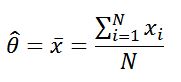
Where:
Xi = individual times for each observation of the sample size “N”
N = number of statistically independent sample observations
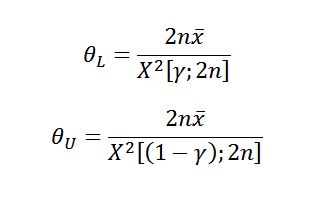
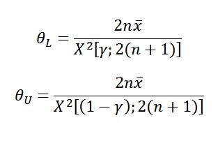
Case 1: In an attempt to put the discussion into perspective, Rolf Sundberg produced a paper titled, “Comparison of Confidence Procedures for Type I Censored Exponential Lifetimes” (Stockholm University, Sweden, 2000) which summarizes seven methods for constructing confidence bounds for time-truncated tests. One of these methods, proposed by Nelson (1982), and advocated also by Cox & Oakes (1984, Sec. 3.4), uses 2n degrees of freedom (n = number of failures) in the Chi-square distribution to calculate both the lower and upper confidence bounds on the MTBF. The equations for calculating the upper and lower bounds for both the one-sided and two-sided cases are:
| Exponential Limits for Time Truncated Test (Case 1) | |
| One-Sided Confidence Interval | Two-Sided Confidence Interval |
 |
 |
This approach is identical to the failure-truncated test case. There are two major issues with this approach. The first is that the 2n assumption basically ignores any test time beyond the last failure from the perspective of confidence bound calculation. The second problem arises in the special case when no failures occur during the course of the test. The 2n degrees of freedom assumption in the Chi-square distribution does not allow for the calculation of any valid confidence bounds in this very realistic zero failure testing scenario.
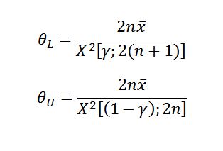
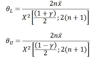
Case 2: A slight modification to this “2n” approach has been advocated in the Department of Defense (DoD). In this approach, MIL-HDBK-338, MIL-HDBK-781 and MIL-HDBK-189 all use “2(n+1)” (i.e., “2n+2”) to calculate the degrees of freedom for the lower MTBF confidence bound and, like the previous approach, use 2n for the upper MTBF confidence bound. The equations for calculating the upper and lower bounds for both the one-sided and two-sided cases are:
| Exponential Limits for Time Truncated Test (Case 2) | |
| One-Sided Confidence Interval | Two-Sided Confidence Interval |
 |
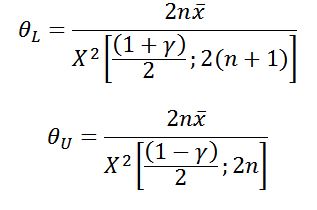 |
This modification does allow for the calculation of a lower confidence bound on the MTBF in the zero failure case (which is important for DoD purposes), but still does not allow for a realistic upper bound calculation.
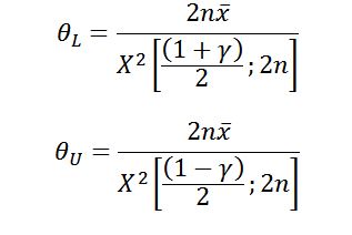
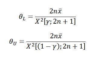
Case 3: Another method, proposed by Cox (1953) and taken up by Lawless (1982), uses “2n+1” for both the lower and upper confidence bounds. This method essentially assumes progression “half-way” to the next failure at the time of test truncation. It also allows confidence intervals to be constructed for the zero failure case. The equations for calculating the upper and lower bounds for both the one-sided and two-sided cases are:
| Exponential Limits for Time Truncated Test (Case 3) | |
| One-Sided Confidence Interval | Two-Sided Confidence Interval |
 |
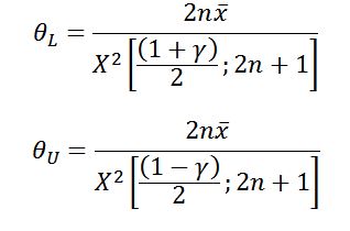 |
Case 4: In yet another approach, Dr. Jorge Luis Romeu, in Selected Topics in Assurance Related Technologies (START) Volume 10, Number 7, “Reliability Estimations for the Exponential Life”, advocates the use of “2n+2” to calculate the degrees of freedom for both the lower and upper MTBF confidence bounds. The equations for calculating the upper and lower bounds for both the one-sided and two-sided cases are:
| Exponential Limits for Time Truncated Test (Case 4) | |
| One-Sided Confidence Interval | Two-Sided Confidence Interval |
 |
 |
This is essentially equivalent to assuming that the next failure is “imminent”. It also permits confidence bounds to be constructed in the zero failure case. This approach is the one incorporated into Quanterion’s System Reliability Toolkit-V and the Quanterion Automated Reliability Toolkit – Enhancing Reliability (QuART-ER) software.
It should be noted that all of the methods described in Case 1 through Case 4 are approximations to the true lower and upper MTBF confidence bounds. Figure 1 & 2 shows the relationship between the two-sided confidence bounds for the different methods. The differences in the calculation of the number of degrees of freedom will result in either wider or narrower confidence intervals. The method using 2n+2 degrees of freedom produces the lowest risk confidence interval, while 2n degrees of freedom (lower and upper) produces the highest risk confidence interval of the four cases. Ultimately, the method that most closely supports your objective and your level of risk aversion is the one that should be used.
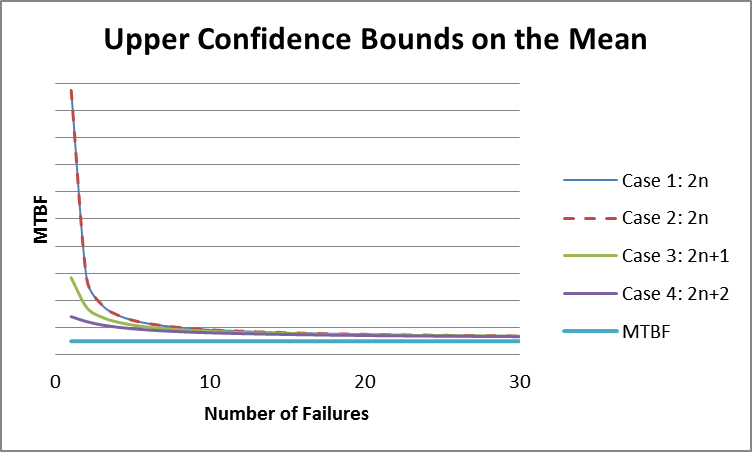 Figure 1: Upper Confidence Bounds for Each Case
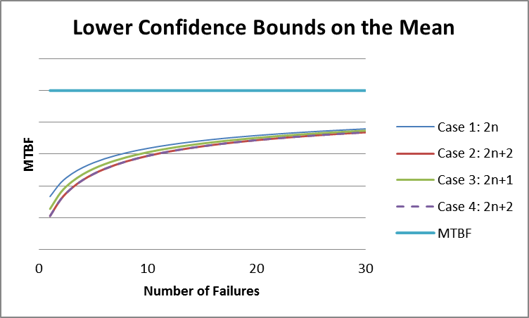 Figure 2: Lower Confidence Bounds for Each Case
It is important to note that the difference between the four cases becomes less and less important as the number of failures in testing grows, and is most critical in zero/low-failure cases. The following example will help to demonstrate the importance of degrees of freedom in zero/low-failure cases.
EXAMPLE
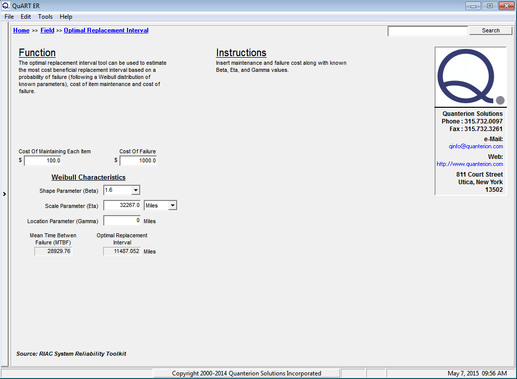
Figure 3 shows the calculated results for a time truncated test with 90% confidence bounds (degrees of freedom = 2n + 2) and a total test time 0f 1000 hours with zero failures. Note that as the failure distribution in this case is assumed to be exponential, the actual number of units on test is not necessary for calculation purposes, only the total test time.
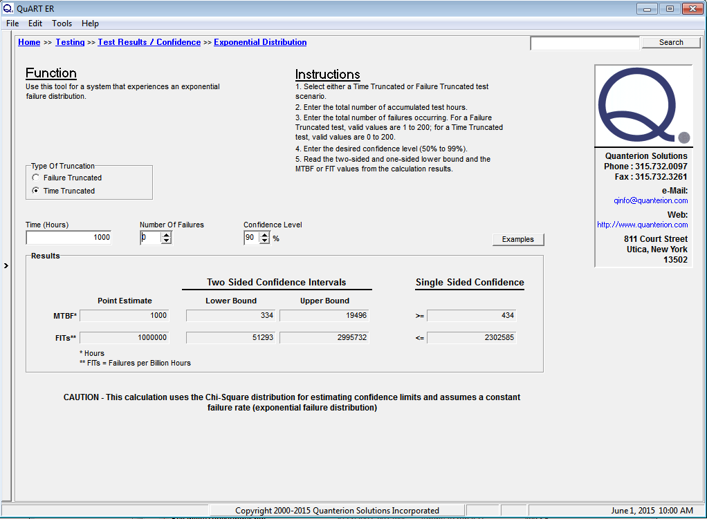 Figure 3: Zero Failure Test Time Calculations
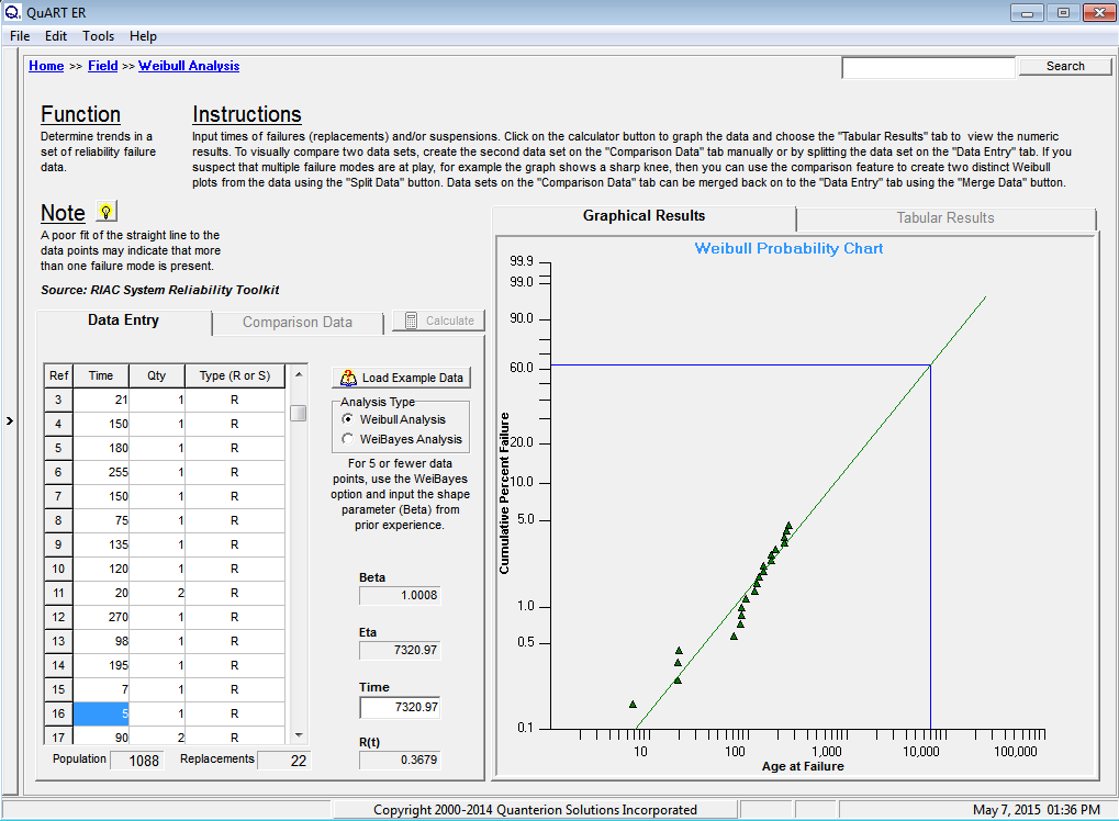
As can be seen from the figure, QuART-ER performs a number of different calculations with the input data. The first calculation is for the system’s MTBF point estimate. In the zero failure case, the assumption that a failure of the system is imminent (n = 1) results in a MTBF = 1000 hours. Note that the calculated MTBF point estimate for the single-failure case shown in Figure 4 is also 1000 hours. In this case, “n” actually does equal 1. In contrast, the lower and upper confidence bound are calculated based on the actual number of failures the system has experienced (zero failure case, n = 0 and single failure case, n = 1). An analysis of the figures clearly shows that upper confidence bounds are indeed calculated in both cases and the resulting magnitudes show the substantial difference between the two scenarios.
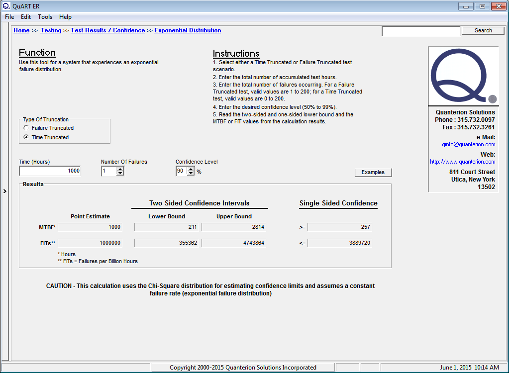 Figure 4: Single Failure Test Time Calculations
As mentioned previously, the DoD has adopted the 2n degrees of freedom method for the upper bound confidence interval which cannot be calculated for the zero failure case. One reason for this is that the DoD uses this type of testing to predict future fielded system performance and the lower bound is all that matters from a reliability prediction perspective. This is not to say that the upper bound prediction has no value in the overall decision-making process.
As an example, consider the following scenario. Suppose that the data in Figure 3 and Figure 4 represent two possible outcomes from early testing of a new system and the design requirement for the system is for a MTBF = 5000 hours within a two-sided 90% confidence interval. The upper confidence bound in the zero failure case of 19,496 hours demonstrates that the MTBF of the system under test still has the “potential” of being met with additional testing time. The upper confidence bound in the single failure case of 2,814 hours demonstrates that the MTBF of the current system design is very “unlikely” to meet the design requirement and further testing would be a waste of money and time. Figure 4 clearly shows that it is time for a reliability improvement effort.
References:
Sundberg, R. “Comparison of Confidence Procedures for Type I Censored Exponential Lifetimes”, Stockholm University, Sweden, 2000.
Nelson, W. “Applied Life Data Analysis”, Wiley: New York, 1982.
Cox, D.R., Oakes, D. “Analysis of Survival Data”, Chapman and Hall: London, 1984.
MIL-HDBK-338B, “Electronic Reliability Design Handbook”, 1998.
MIL-HDBK-781A, “Handbook for Reliability Test Methods, Plans and Environments for Engineering, Development, Qualification and Production”, 1996.
MIL-HDBK-189, “Reliability Growth Management”, 2011.
Cox, D.R., “Some Simple Approximate Tests for Poisson Variates”, Biometrika, vol. 40, pp. 354-360, 1953.
Lawless, J.F., “Statistical Models and Methods for Lifetime Data”, Wiley: New York, 1982.
Romeu, J. L., “Reliability Estimations for the Exponential Life”, Reliability Analysis Center (RAC), Selected Topics in Assurance Related Technologies (START), Volume 10, Number 7, 2003.
“System Reliability Toolkit – V: New Approaches and Practical Applications”, Quanterion Solutions Inc., 2015.