In simplest terms, an item fails when a stress to which it is subjected exceeds the corresponding strength. In this sense, strength can be viewed as “resistance to failure”. Good design practice is such that the strength is always greater than the expected stress. The safety factor “η” can be defined in terms of strength and stress as follows:

equation-1
For example, suppose that the stress on a component is 2500psi and its strength is 4000psi. The safety factor “η” would be calculated as 4000psi/2500psi = 1.6. At first glance, it might be concluded that since the safety factor is greater than 1 that the item will not fail due to this stress. While this would be true if stress and strength could be viewed as simple point values, in reality variability exists around both of these parameters. To illustrate this point, suppose, in the above example, the stress and strength were normally distributed about the means of 2500psi and 4000psi with standard deviations of 500psi and 400psi, respectively. A plot of these distributions is shown in Figure 1.

figure-1
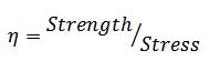
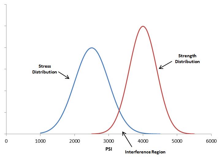
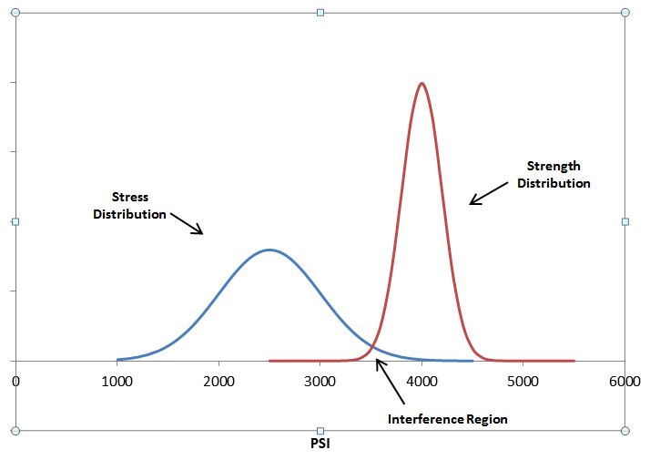
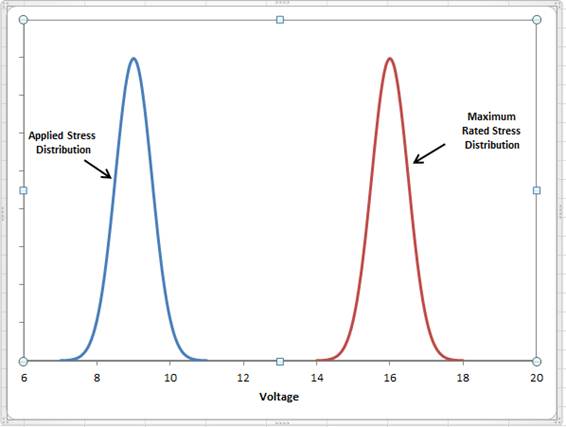
Figure 1: Stress and Strength Distribution Example
It is evident that while the mean strength is greater than the mean stress, there exists a region where the distributions overlap and the stress can actually exceed the strength and lead to part or material failure. This region is referred to as the “Interference Region”. From a “qualitative perspective”, the existence of this interference region implies there is a probability of failure for the design.

If stress and strength are normally distributed random variables and are independent of each other, then the standard normal distribution and Z tables can be used to “quantitatively” determine the probability of failure. First, the Z-statistic is calculated as follows:

equation-2
where “μS” is the mean of the strength distribution, “μsapp” is the mean of the stress distribution, “σS2” is the variance of the strength distribution and “σsapp2” is the variance of the stress distribution. Using the Z value table for a standard normal distribution, the area above the calculated Z-statistic is the probability of failure.

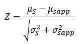
If stress and strength are not normally distributed, other techniques (such as Monte Carlo simulation) may be used to determine the probability of failure.

Calculating the probability of failure using the distributions shown in Figure 1 and the related data we have:

equation-3
Using the Z-value table for a standard Normal distribution, the area above a Z value of 2.34 (2.34 standard deviations) is 0.0096. Therefore, the probability of failure is 0.96%. Likewise, the reliability is 1-0.0096 = 0.9904 or 99.04%.

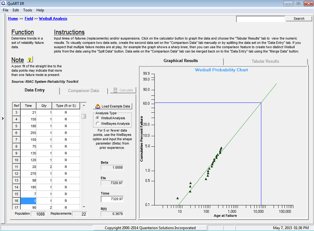
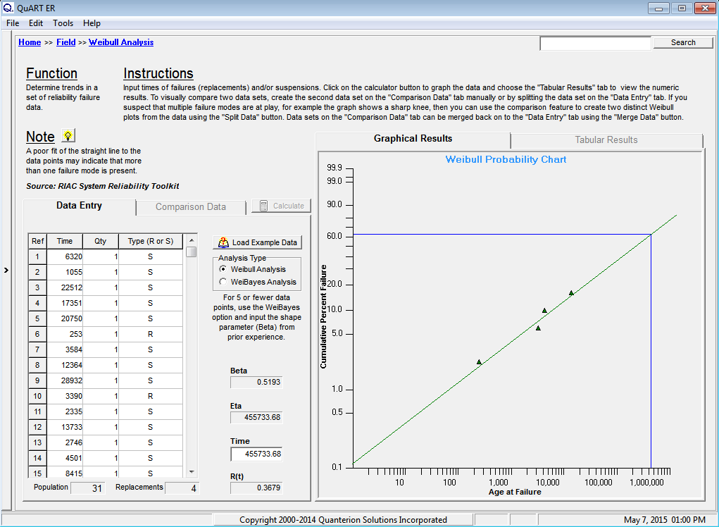
The Interference Stress/Strength Analysis calculator in the Quanterion Automated Reliability Toolkit – Enhanced Reliability (QuART-ER) tool can be used to perform the calculations. The mean and standard deviation of the stress and strength distributions are entered in the appropriate fields and the resulting probability of failure and reliability are displayed as shown in Figure 2.

figure-2
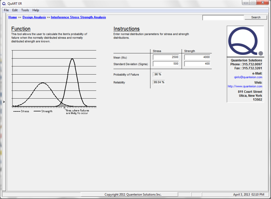
Figure 2: QuART-ER Interference Stress/Strength Analysis Calculator
As shown in the above example, although the mean strength is greater than the mean stress, and the resulting safety factor is greater than 1, failure is not precluded. Indeed, the probability of failure is on the order of 1%. If this probability of failure is unacceptable, then several measures can be taken to reduce it. These measures include increasing the mean strength by choosing another component or redesigning the current one, decreasing the stress by redesigning an electronic circuit, lowering vibration levels, reducing temperature, etc., and decreasing the variation in either or both of the strength and stress distributions. All of these methods will separate the strength and stress distributions and reduce the area of the interference region.

For example, suppose it was possible through careful control of manufacturing processes to reduce the standard deviation of the component’s strength from 400 psi to 200 psi, with the other parameters remaining the same. The stress and strength curves would then be as shown in Figure 3.

figure-3
Figure 3: Stress and Strength Distribution Example – Reduced Strength Variability
Using the QuART-ER Interference Stress/Strength Analysis calculator, the probability of failure is now calculated to be 0.27%, and the reliability is calculated to be 99.73%.

Summary

A brief overview of Interference Stress/Strength Analysis has been provided here, along with sample calculations using Quanterion’s QuART-ER Stress/Strength Calculator. This topic is also covered in the Quanterion-authored Reliability Information Analysis Center (RIAC) publication “System Reliability Toolkit” and is included in the “Reliability-101” training program.