Probability and Statistics for Reliability: An Introduction

Painful as it is to many of us, the generally desirable product characteristicReliability is heavily dependent on Probability and Statistics for measuring and describing its characteristics. This edition of Reliability Ques will only be the tip of the iceberg in this regard. Let’s start with a few basics:

Failure Distribution: this is a representation of the occurrence failures over time usually called the probability density function, PDF, or f(t).
Cumulative Failure Distribution: If you guessed that it’s the cumulative version of the PDF, you’re correct. It’s called the CDF, or F(t)
Reliability: If we can call the CDF the unreliability of a product, then 1-F(t) must be the reliability.

With these basics, an important part of reliability is identifying, understanding, and optimizing the type of statistical distribution that represents the product. The following are a few common examples:

Normal Distribution: the most common distribution usually representing wearout situations (2 parameter).
Exponential Distribution: a one parameter distribution usually used for electronic products, or products where there are all sorts of distributions tending to combine to a constant hazard rate.
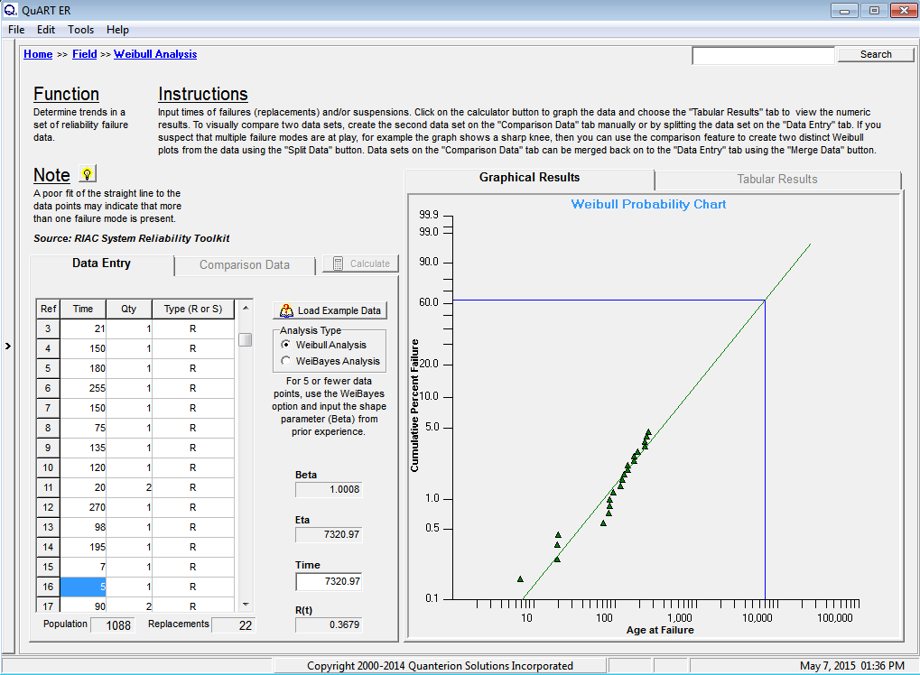
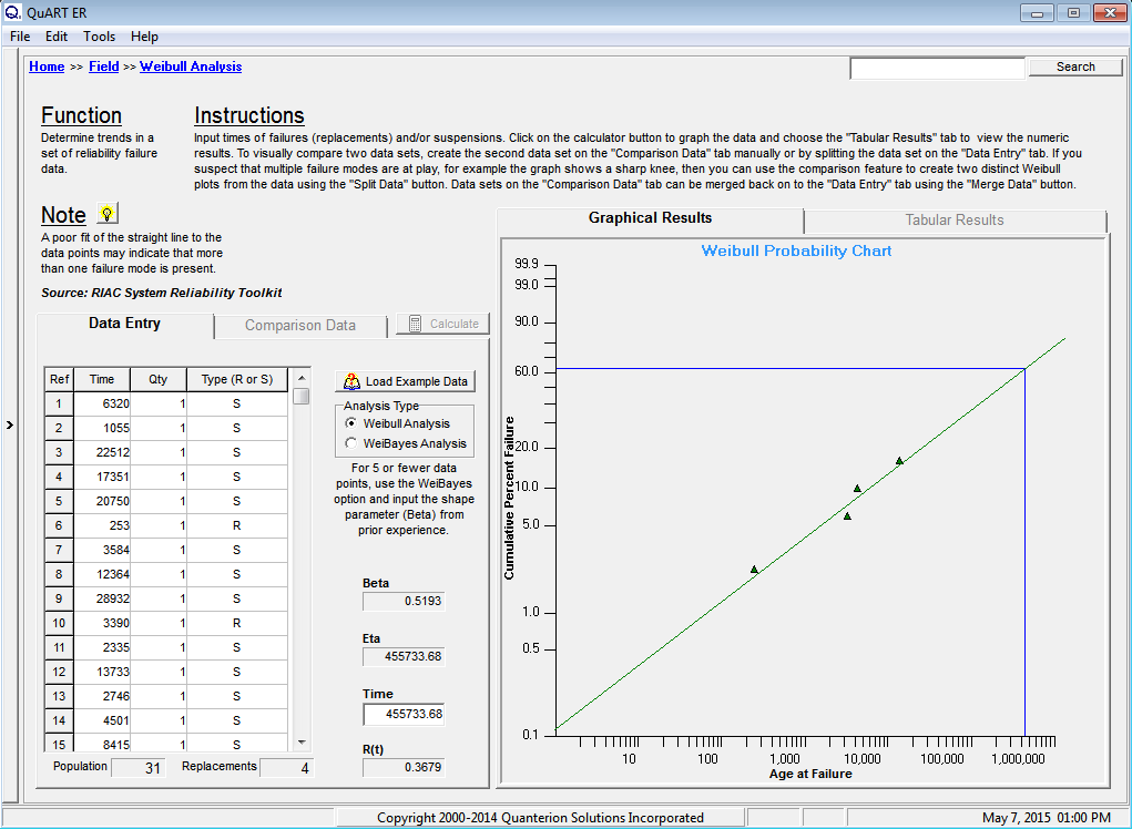
Weibull Distribution: can be used to represent a number of other distributions such as the Normal, the Exponential, and others (usually 2 parameter but can be 3 parameter). The Weibull can be used to represent the three regions of the classic reliability “Bathtub” curve: (Region 1) the decreasing failure rate associated with infant mortality, (Region 2) the constant failure rate of useful life, and (Region 3) the wearout period of increasing failure rate. The Weibull parameters β, called the Weibull Shape Parameters, for the three Bathtub regions are respectively <1.0, =1.0, and >1.0.
Binomial Distribution: used to represent situations where there are two possible outcomes, success or failure and the probability of one of the types of outcomes is known.

So far, so good, for many of you this may be a refresher but what are some other applications?

Poisson Distribution: used to determine the likelihood of a number of events occurring in a set of trials if the likelihood of an individual event is known.
Hypergeometric: used to determine the likelihood of exactly “x” events in a sample of “y” given that there “m” of the events in the total population of “n.” This distribution is similar to the Binomial.
Geometric: used to determine the likelihood of success at the “xth” trial when the probability of an individual event is known.

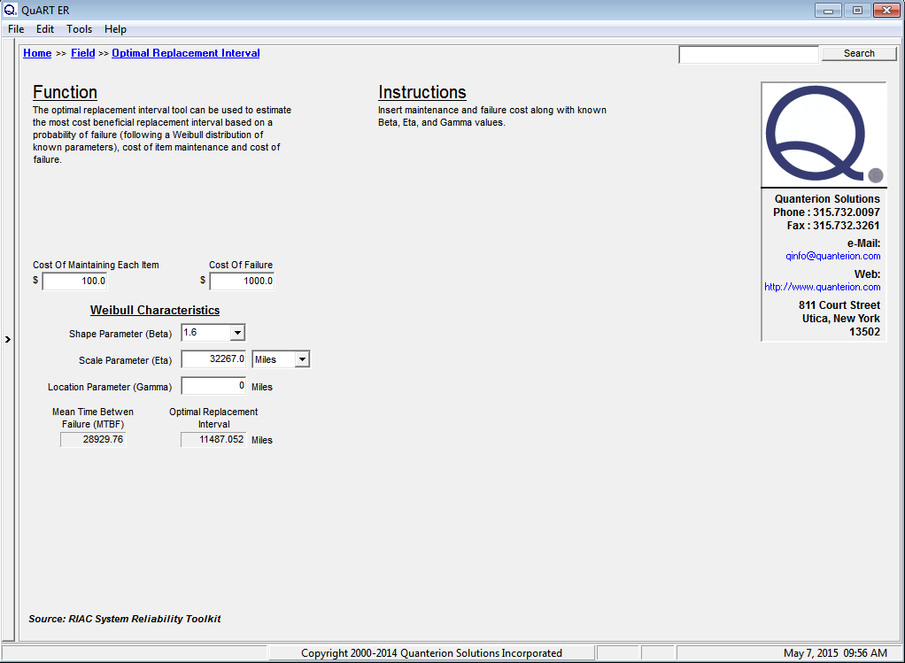
Great, now drag out the statistics tables. Sorry to disappoint, we have an easier way for FREE. The QuART PRO and QuART ER software suites include demo versions of the tools to do the calculations for all the above distributions without cracking a book open. Let’s give it a try with some examples:

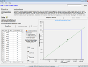
If a particular type of resistor’s resistance is normally distributed with a mean of 100 ohms and a standard deviation of 5 ohms, what’s the probability of getting a resistor with a resistance less than 85 ohms? Enter the data in QuART PRO to arrive at a probability of 0.13%, or 0.0013.
If the required reliability for a mission of 100 hours is 99.9%, what must the failure rate (assumed constant) be for the electronic product to meet the requirement? Enter the number of hours and iterate the failure rate until the Reliability equals 99.9%. The failure rate will be 0.00001 failures/hour, or in more common terms 10 failures/10⁶ hours.
What’s the reliability of a shaft at 1,000 hours if its Weibull Shape Parameter is 1.7 and its Weibull Characteristic Life (point at which 63.2% of population has failed) is 700 hours? Read a reliability of only 15.98%.
In a bin of parts, where 10% are known to be bad, what’s the probability of selecting 8 out of 10 that are good? Read the result for 10 minus 8, or 2 bad parts as 19.37%.
What’s a developer’s risk of having his product with a true Mean-Time-Between-Failure (MTBF) of 500 hours rejected in a test of 1000 hours where the acceptable number of failures in the test is 3 or less? Trick question? Not really. Let’s make some adjustments before we go to the QuART PRO Poisson calculator. First, if the time is 1000 hours, and the MTBF is 500 hours, we’d expect 2 failures.
Our first calculation shows that the probability of 3 failures is 18.04%. Similarly, for 2 failures it’s 27.07%, for 1 failure it’s 27.07%, and for no failures it’s 13.53%. Therefore, the probability of 3 failures or less is the sum, which is 85.71%. So, if the probability of 3 or fewer failures is 85.71%, then the probability of 4 or more is 14.29%, which is the developer’s risk of having his product rejected.