A reliability model represents a clear picture of your product’s functional interdependencies providing a means to trade-off design alternatives and to identify areas for design improvement. The models are also helpful in:
- Identifying of critical items and single points of failure
- Allocating reliability goals to portions of the design
- Providing a framework for comparing estimated reliability to product goals
- Trading-off alternative fault tolerance approaches
Reliability models are derived from, and traceable to, functional requirements. They represent the required modes of operation, the duty cycles, and are consistent with a specified definition of what constitutes a product or system failure.
Repairable Versus Non-Repairable Systems
Systems can be grouped into two categories: repairable or non-reparable types. For repairable systems the measure of interest is often “effective” mean-time-between-failure, sometimes termed mean-time-between-critical-failure (MTBCF). For non-repairable systems (e.g., many spacecraft systems) or systems with some critical mission length, probability of success for a given mission time, is a more common measure.
Computation of System Reliability
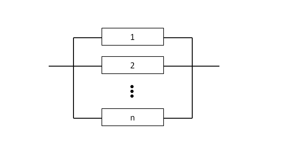
For non-repairable systems, it is usually desirable to know what the probability of success (system reliability) is over a given period of time. The basic steps involved in developing a system reliability model are first to define what is required for mission success and second to define the probability of being in each possible system state (good or failed). The probability of successful system operation is the sum of the probabilities of being in a good state. The following is an example of modeling a set of dual redundant CD-ROM drives. This example assumes perfect switching between drives. The definition of system success: one of the two disk drives must work.
The possible states of the individual drives and the composite two drive “system” are shown below in Table 1 (G=Probability Drive is Good, F=Probability Drive Has Failed).
| State | Drive 1 | Drive 2 | Probability of System Being in State |
| A | G | G | [G][G] |
| B | F | G | [F][G] |
| C | G | F | [G][F] |
| D | F | F | [F][F] |
The probability of successful system operation (one of the two disk drives operating) is equal to the probability of being in either states A, B, or C above. Therefore:
P(Success) = P(A) + P(B) + P(C)
P(Success) = [G][G] + [F][G] + [G][F]
Where:
[G] = Probability that the relevant item is “functional” and operating
[G] = 1 – [F]
[F] = Probability that the relevant item is not functional or operating
[F] = 1-[G].
Thus far, no assumptions regarding the failure distributions have been made. Any probabilistic failure distribution can be substituted for “G” and “F” above; however, the most widely accepted failure distribution for electronics is the exponential (i.e., constant instantaneous failure rate (hazard function, λ). The reliability function in the exponential case is: R(t) = e-λt, where λ is the failure rate and t is the period of time over which reliability is measured. The probability of failure is F = 1 – R(t). Thus to determine the probability of success assuming the exponential case, e-λt and 1-e-λt are substituted for G and F, respectively. These substitutions are shown in Table 2.
| State | Drive 1 | Drive 2 | Reliability | |
| A | e-λt | e-λt | [e-λt][e-λt] | e-2λt |
| B | 1-e-λt | e-λt | [1-e-λt][e-λt] | e-λt – e-2λt |
| C | e-λt | 1-e-λt | [e-λt][1e-λt] | e-λt – e-2λt |
| D | 1-e-λt | 1-e-λt | [1-e-λt][1-e-λt] | 1 – 2e-λt + e-2λt |
The probability of the composite drive “system” being in a functionally working state (i.e., states A, B, or C) is:
R(t) = P(A) + P(B) + P(C)
R(t) = e-2λt + e-λt – e-2λt + e-λt – e-2λt
R(t) = 2e-λt – e-2λt
If we are interested in the probability of success at the one year point and we know from historical field data that each drive has an MTBF of 25,000 hours, or a failure rate of 40 failures per 106 hours (FPMH), then the probability of success is:
R(t) = 2e-(.00004)(8760) – e-2(00004)(8760)= 0.91 or 91%
Where:
t = (1 Yr.)(8760 Hr/Yr.) = 8760 Hours
Failure Rate (λ) = 1/MTBF = 1/25000 = .00004 Failures/Hour
This 91% probability of success is a 30% improvement over the probability of success for a single drive, which is : R(t)=e-λt=R(8760)=e-(.00004)(8760)=0.70, or 70%. However, it should be noted that cost increases for this added reliability in terms of hardware acquisition costs, software routines to access the spare drive, as well as other related costs such as system size, weight and power consumption. Redundancy calculations like these can be easily carried out using tools like theQuanterion Automated Reliability Toolkit (QuART).
Computation of Mean-Time-To-Failure
For a non-repairable system, it is often desirable to know the mean-time-to-failure for a system rather than simply the probability of success. MTTF can be determined by integrating the reliability function from zero to infinity:
Computation of Mean-Time-Between-Failure
For a repairable disk drive configuration periodically maintained, the general expression for Effective MTBF is as follows:
where T represents the unattended period of operation (i.e., after every T hours a maintenance team visits the system and repairs all failures) according to some maintenance script. R(t) in the equation above is the derived reliability function based on possible good and failed states, and R(T) is the same function evaluated at t=T.
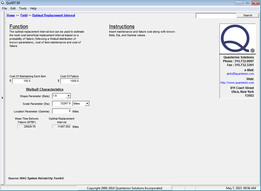
If the maintenance concept for the redundant disk drives is for periodic maintenance once every year, then T=8760 hours. Substituting T=8760 hours into the above equation and integrating:
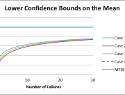
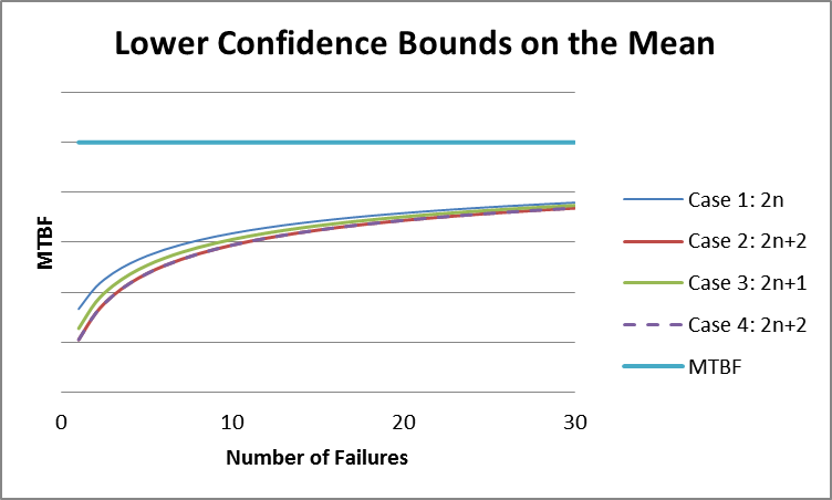
Figure 1 – Effective MTBF for Maintained and Non-maintained Systems
System models vary from relatively simple to highly detailed, taking into account things such as duty cycles, service life limitations, wear out items, varying environments, and dormant conditions. The scope of the model usually depends on the type and amount of information available for use and the criticality of the system under consideration.
Example System Reliability Model
Figure 2 presents a simple reliability block diagram of a system. Table 3 summarizes a hypothetical assembly level set of failure rate data.
Figure 2- Hypothetical Personal Computer System Model
| Unit | Qty | Failure Rate (FPMH) | Data Source | Data Source Environment | Environmental Adjustment Factor | Total Failure Rate (FPMH) |
| CD-ROM Drive | 2 | 40 | Field | Office | 1 | 80 |
| 3.5″ Disk Drive | 3 | 10 | Handbook | Office | 1 | 30 |
| Hard Drive | 1 | 35 | Vendor Test | Office | 1 | 35 |
| CPU Board | 1 | 4 | Field | Aircraft | 0.25 | 1 |
| Keyboard | 1 | 10 | Field | Office | 1 | 10 |
| Monitor | 1 | 40 | Field | Aircraft | 0.25 | 10 |
| Modem | 1 | 3 | Handbook | Office | 1 | 3 |
| Total (Failures Per Million Hours) | 169 | |||||
It should be noted that the adjustments shown in Table 3 are to account for the application environment (i.e., aircraft versus ground). Other adjustments can be made to account for different conditions, such as duty cycle, temperature, part screening and soft error rate (note, this simplistic model assumes no failure rate contribution due to the occurrence of soft errors). Adjustment factors such as these are available in QuART. Common adjustment factors for a component’s electrical, thermal and mechanical stresses exist in MIL-HDBK-217. Thus for this example, the series failure rate, which is simply every “box” in series (all must work) is 169 failures per million hours (FPMH). Taking the reciprocal of this results in a mean-time-between-failure (MTBF) of 5917 hours.
It can easily seen from the above discussion the value of establishing a reliability model for a product or system in order to fully understand its limitations, and to trade off design alternatives. While the examples presented are somewhat simple, the methodology can be easily extended using more complex relationships such as those of Appendix A. For systems with more complex redundancy schemes and other fault tolerance features that cannot easily be reduced to a closed form model, system modeling and simulation software packages must be employed. These packages typically provide the ability to mimic a system’s behavior over time by using a random number generator to generate events (failures and repair actions) and track resulting system state over time.