The goal of improving system reliability often presents a design paradox; “mission” reliability cannot be increased without simultaneously decreasing “logistics” reliability. When faced with the challenge of a system that has inadequate reliability to meet specification requirements, hardware redundancy is often implemented, leading to an improvement in one metric while degrading others.
For example, let’s say the radar system shown in Figure 1 has a requirement for a 10,000 hour mean-time-between-failure (MTBF). In order to determine if this goal can be achieved, failure rate data on each item is determined, as shown in Table 1. If an exponential failure distribution is assumed, indicating that failures are expected to occur at random times (e.g., no sudden wearout), then item failure rates can be added to estimate the overall radar system failure rate. The failure rates for the individual items are usually either obtained from field failure history (more desirable) or from generic handbook models (less desirable), such as MIL-HDBK-217, Reliability Prediction of Electronic Equipment. As shown by the summation of failure rates in Table 1, this particular design has an overall system failure rate of 113 failures per million hours (FPMH), or an MTBF of 8,550 hours, and thus does not meet the 10,000 hour requirement. Because there is no redundancy in the design, the “logistics,” or “series” MTBF is the same as the “mission” MTBF, which is 8,550 hours.
Figure 1: Radar Reliability Block Diagram Model
| Item Number | Item | Quantity | Failure Rate (FPMH) |
|---|---|---|---|
| 1 | Power Supply | 1 | 20 |
| 2 | Transmitter | 1 | 36 |
| 3 | Antenna | 1 | 3 |
| 4 | Receiver | 1 | 22 |
| 5 | Signal Processor | 1 | 14 |
| 6 | Environmental Control Unit | 1 | 18 |
| Total Failure Rate | 113 | ||
| Mean-Time-Between-Failure (Hours) | 8,850 | ||
Ideally, when faced with this situation, it is most desirable to improve system reliability through actions that do not increase the amount of hardware in the system, such as:
- Design simplification to reduce the number of components
- Component derating, which requires that parts be operated at stress levels lower than their ratings
- Improved cooling to lower component operating temperatures
- Use of higher quality parts
If actions such as those listed above still do not provide a sufficient increase in system reliability, then redundancy must be added. Redundancy has the advantage of providing large increases in MTBF, especially for maintained systems when failed redundant items are promptly repaired. However, redundancy has the disadvantage of adding more hardware, which adds weight, power consumption and sometimes significant design complexity for failure sensing and switching circuits. Redundancy also has the disadvantage of degrading “series” or “logistics” MTBF because more hardware will create a higher demand for maintenance.
If we revise our radar system design shown in Figure 1 to add a redundant power supply as shown in Figure 2, we can meet our 10,000 hour requirement, as shown in the revised calculations of Table 2. As Table 2 indicates, there are now two system failure rate calculations, an effective “mission” failure rate, which takes into account the effects of redundancy, and a “logistics” or “series” failure rate which accounts for the failure rate contribution of all hardware. Thus, while the series MTBF has decreased from the 8,850 hours calculated in Table 1 to 7,519 hours calculated in Table 2, the effect of adding redundancy has increased the “mission” MTBF, sometimes termed mean-time-between-critical-failures (MTBCF), from 8,850 hours to 10,752 hours.
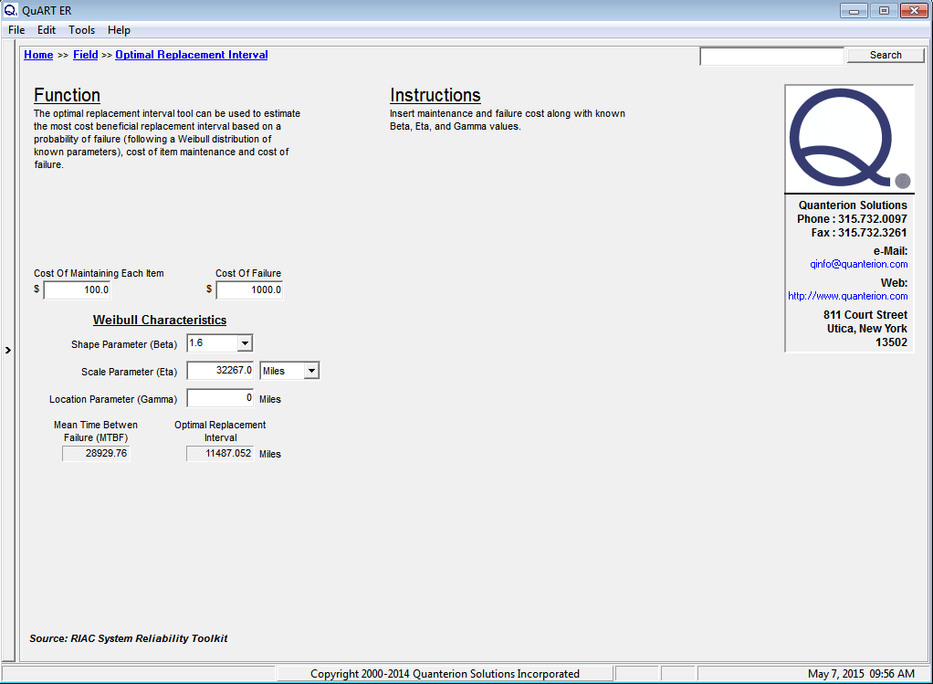
This result assumes a mean-corrective-maintenance-time of eight hours, which means that a failed power supply will be repaired on average within eight hours, providing for an effective failure rate of the one-of-two power supply configuration of 0.0064 FPMH, as shown in Table 2. These calculations can be performed using the redundancy equations summarized in a previous Reliability Ques article “Understanding Your Product Through Reliability Modeling” or as we have done here, by using the handy redundancy calculator included in the licensed version of the Quanterion Automated Reliability Toolkit (QuART) shown in Figure 3. Free demo versions of both QuART Pro and QuART ER are available for download.
Figure 2: Revised Radar Reliability Block Diagram Model
| Item Number | Item | Quantity | Number Required | Failure Rate per Item (FPMH) | Effective Failure Rate (FPMH) | Logistics/Series Failure Rate (FPMH) |
|---|---|---|---|---|---|---|
| 1 | Power Supply | 2 | 1 | 20 | 0.0064 | 40 |
| 2 | Transmitter | 1 | 1 | 36 | 36 | 36 |
| 3 | Antenna | 1 | 1 | 3 | 3 | 3 |
| 4 | Receiver | 1 | 1 | 22 | 22 | 22 |
| 5 | Signal Processor | 1 | 1 | 14 | 14 | 14 |
| 6 | Environmental Control Unit | 1 | 1 | 18 | 18 | 18 |
| Total Failure Rate | 93.01 | 133.00 | ||||
| Mean-Time-Between-Failure (Hours) | 10,752 | 7,519 | ||||

Figure 3: QuART Redundancy Calculator